Beginning from First Principles. Understanding the seismic characteristics of scaled accelerograms requires us to visit the mechanics of earthquake processes. By visiting the earthquake mechanics, per the author’s opinion, we can gain insights into the physics of the scaling process. Such a comprehension of the physics will further enable us to inform, in a better way, about the safety of infrastructure under strong earthquakes by attributing some character to the scaling procedure. As discussed in the Previous Post, earthquake safety assessment of infrastructure may routinely rely on scaling accelerograms.
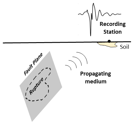
Earthquake Mechanics. The earthquake process and its effects, as summarized in the figure below, can be divided into three components: (1) rupture on the fault plane and generation of seismic waves; (2) propagation (which leads to dissipation and attenuation) of seismic waves through the medium surrounding the fault plane; (3) reception of the seismic waves at a recording station in the form of an accelerogram.
The ground motion at a site caused due to rupture on the fault plane is mathematically described by the Representation Theorem in seismology, which is derived from elastodynamical priciples (or the dynamic equations of motion for a deformable body). The Representation Theorem can be described as a cornerstone of seismology, providing theoretical as well as observational insights on earthquakes. The definition of moment magnitude for an earthquake and the development of hybrid ground motion simulation methods find their roots in the Representation Theorem. Whenever an earthquake occurs, earthquake monitoring agencies may rely on the Representation theorem to infer the slip distribution over the fault plane given the ground motion at a site. Owing to this key role the Representation theorem plays in seismology, it will be used as means to understand the seismic characteristics of scaled accelerograms.
(Informal) Representation Theorem. Ground motion at a site on the earth’s surface, using the Representation Theorem, can be expressed as a function of three ingredients: (1) fault strength and geometry; (2) rupture amplitude over the fault; and (3) impulse response of the propagating medium. The figure below presents the Representation Theorem in an informal fashion. For the formal definition, refer to equation (2.41) in Aki and Richards 2002.
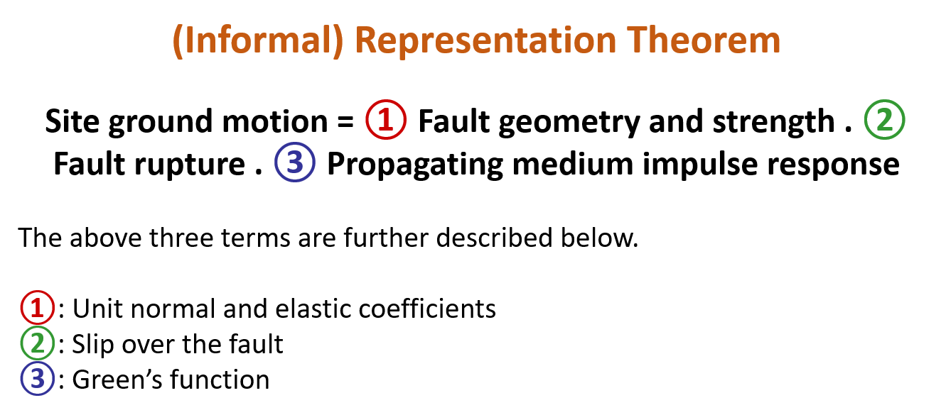
Observing the Representation Theorem in the above figure, it is noted that ground motion at a site can be kinematically determined once the fault rupture (or slip over the fault plane) is known. This fault rupture, as seen in the figure above, is first multiplied with fault’s elastic coefficients and unit normal (which represent the strength and geometry of the fault, respectively) to convert displacements to forces. Next, the composite of terms (1) and (2)–which is in terms of a force–is multiplied with the impulse response of the propagating medium to give the ground motion at the site. This impulse response term (3 in the figure) is the ground motion observed at the site for an unit force applied on the fault plane, and it is also called the Green’s function. It is, therefore, intuitive that the product of the Green’s function and the force applied on the fault plane (product of terms 1 and 2) will give us the required ground motion. These three terms which makeup the Representation Theorem are discussed in further detail.
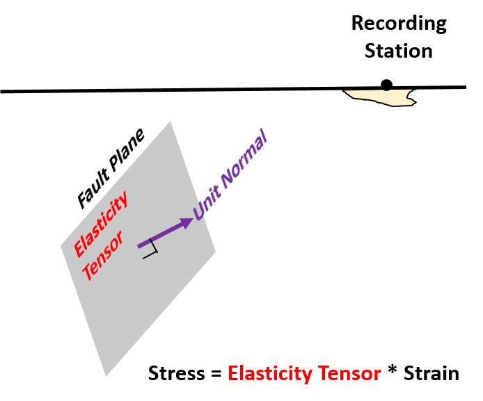
(1) Fault Strength and Geometry. Strength of a fault is described by the elastic properties of the rock medium surrounding it. Elastic properties, in Structural Engineering language, are the Young’s, Rigidity, and Bulk moduli. However, these moduli can be mathematically derived from what is called the Elasticity tensor. The Elasticity tensor is a fourth order tensor describing the relationship between material stresses and strains in all three directions. Elasticity tensor depicts the strength of the fault in the Representation Theorem. Geometry of the fault-plane is described by a unit normal vector. The unit normal is a vector normal to a plane whose magnitude is unity. The figure below presents the elasticity tensor and the unit normal of a fault-plane. As will be seen in the Next Post, both these quantities play a key role in setting up the problem of developing the accelerogram amplitude scaling seismology.
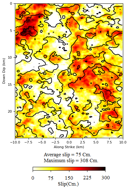
(2) Fault Rupture (Slip). Most earthquakes are caused by rupture or slip over the fault which is described as the relative displacement of the two faces of a fault. The fault rupture term quantifies the amount of relative displacement both as a function of the spatial extent over the fault and time. The figure below presents an example of the fault rupture term where relative displacements over a fault averaged in time are depicted. It is noted that these displacements vary considerably over the fault-plane. Rupture distributions such as the below are obtained using finite fault inversion which is an active area of seismology research, owing to the significant uncertainties that are encountered during the inversion process. As will be seen in one of the following posts, the fault rupture term plays a crucial role in determining the magnitude and the distance of a scaled accelerogram.
(3) Propagating Medium Impulse Response (Green’s Function). Once there is rupture over the fault plane, the propagating medium is responsible for transimitting this rupture to the site (or recording station). The strength of the recorded ground motion depends on the propagating medium as much as it does on the fault rupture. The propagating medium response is elegantly represented by the Green’s function. Green’s function is the ground motion at a site for a unit force applied on the fault plane. The magitude of this ground motion depends both on the direction of the applied force and the direction of recording. Green’s function, therefore, is a second order tensor. The ij component of this tensor is the ground motion in direction j with force applied on the fault plane in direction i. The figure below presents an example of a component in the Green’s function tensor.
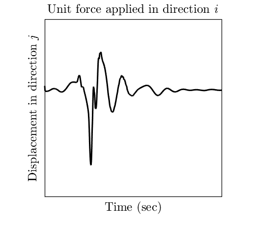
Small magnitude earthquakes can be regarded as impulsive point sources (or as a point load acting at the source). The ground motions from such small earthquakes can be treated as empirical Green’s functions which are widely used for simulating synthetic ground motions from large earthquakes.
In the Next Post, the terms which make up the representation theorem will be investigated in relation to understanding the seismology of accelerogram amplitude scaling.
To cite this page: Dhulipala, S.L.N. (2018) What is the Seismology of Accelerogram Amplitude Scaling? (in review)

This work is licensed under a Creative Commons Attribution-NonCommercial 4.0 International License.